Tuesday, 24 December 2013

SVM - Support Vector Machines


                                                  How To Workout SVM Algorithm


In machine learning, support vector machines (SVMs, also support vector networks) are supervised learning models with associated learning algorithms that analyze data and recognize patterns, used for classification and regression analysis. The basic SVM takes a set of input data and predicts, for each given input, which of two possible classes forms the output, making it a non-probabilistic binary linear classifier. Given a set of training examples, each marked as belonging to one of two categories, an SVM training algorithm builds a model that assigns new examples into one category or the other. An SVM model is a representation of the examples as points in space, mapped so that the examples of the separate categories are divided by a clear gap that is as wide as possible. New examples are then mapped into that same space and predicted to belong to a category based on which side of the gap they fall on.
More formally, a support vector machine constructs a hyper plane or set of hyper planes in a high- or infinite-dimensional space, which can be used for classification, regression, or other tasks. Intuitively, a good separation is achieved by the hyper plane that has the largest distance to the nearest training data point of any class (so-called functional margin), since in general the larger the margin the lower the generalization error of the classifier.

1.1 SVM Binary Classification Algorithm


Example 1:

   
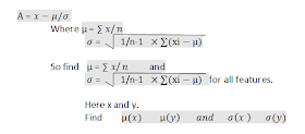
Step 1:Normalize the given data by using the equation


Step 2: Compute Augmented matrix   [A  -e]. ie Augment a "-1" column matrix to A.


Step 3: Compute  H = D[A -e]
where D is a diagonal matrix with classes. here it is 1 and -1.

        D × [A  -e] = 


        HTH


Step 4 : Compute U = V ×[I –H[I/V + HTH]-1 HT]×e
                Where I = Identity Matrix   
                                V = Order of HTH with value 0.1


Step 5: Find  w and gamma  = 0.                
                                                                                             
Step 6: Find w trans * X -gamma. Find for all features
  eg: X= Column_matrix{x,y}


           Result of SVM Traning


Step 7: Compare sign(wT*x -gama ) with the actual class label.
You can notice that 3rd , 5 th and 9 th class labels are misclassified.
ie
After Traning the dataset , the below datapoints

           5     9   falls in class label -1
           8     7   falls in class label -1
           and
           8     5   falls in class label 1.


Misclassification in 3 datapoints 3 rd 5 th and 9 th.
Acurracy is 70%.

Saturday, 21 December 2013

Decision Tree Algorithm


How To Workout Decision Tree Algorithm


Decision Tree Induction is the learning of decision trees from class-labeled training tuples. A decision tree is a flowchart-like tree structure, where each internal node (nonleaf node) denotes a test on an attribute, each branch represents an outcome of the test, and each leaf node (or terminal node) holds a class label. The topmost node in a tree is the root node.

During the late 1970s and early 1980s, J. Ross Quinlan, a researcher in machine learning, developed a decision tree algorithm known as ID3 (Iterative Dichotomiser). This work expanded on earlier work on concept learning systems, described by E. B. Hunt, J. Marin, and P. T. Stone. Quinlan later presented C4.5 (a successor of ID3), which became a benchmark to which newer supervised learning algorithms are often compared. In 1984, a group of statisticians (L. Breiman, J. Friedman, R. Olshen, and C. Stone) published the book Classification and Regression Trees (CART), which described the generation of binary decision trees. ID3 and CART were invented independently of one another at around the same time, yet follow a similar approach for learning decision trees from training tuples. These two cornerstone algorithms spawned a flurry of work on decision tree induction. ID3, C4.5, and CART adopt a greedy (i.e., nonbacktracking) approach in which decision trees are constructed in a top-down recursive divide-and-conquer manner. Most algorithms for decision tree induction also follow such a top-down approach, which tarts with a training set of tuples and their associated class labels. The training set is recursively partitioned into smaller subsets as the tree is being built.

Problem 1:


Iteration 1:

Find gain for class: Play
Calculate the no of yes  and no 
          No – 5
          Yes – 9
Total observation – 14

           Entropy([9,5]) = (-9/14 log 9/14 – 5/14 log 5/14)/log 2 = 0.940


Then find the gain for all instance.

          EntropyOutlook([2,3],[4,0],[3,2]) = 5/14(-2/5 log 2/5 – 3/5 log 3/5) + 4/14(-4/4 log 4/4) + 5/14(-3/5 log 3/5 – 2/5 log 2/5) /log 2

          EntropyTemp([3,1],[4,2],[3,1])/log 2
          EntropyHumidity([4,3],[6,1])/log 2
          EntropyWindy([2,6],[3,3])/log 2

Therefore
          gain(outlook)  = Entropy([9,5]) – EntropyOutlook([2,3],[4,0],[3,2])=0.247
          gain(Temp)       = 0.029
          gain(humidity)   = 0.152
          gain(windy)      = 0.048

Find which is having highest gain and it will be taken as the root node.

So here in overcast all the leaf nodes are yes therefore we don't have a further recursion in that.You can delete the entire row which is having overcast as outlook or else continue with the same table.


Iteration 2:

Now we need to identify what all nodes can come under oulook -> Sunny and outlook -> Rainy.
First look for the case of Sunny. Sort out the master table to a child table which comprises only Sunny entry.


Calculate the no of yes  and no 
          No - 3
          Yes - 2

          Entropy([3,2])        = 0.97095

          gain(Temp)       = 0.57095
          gain(humidity) = 0.97095
          gain(windy)       = 0.419973


Find which is having the highest gain
          gain(humidity) = 0.97095


So humidity comes under Sunny
New tree becomes
 

From the above diagram all leaf node is same . Therefore no iteration with in humidity so remaining left out is Rainy.


Iteration 3:


Now we need to identify what all nodes can come under oulook -> Rainy .
Sort out the master table to a child table which comprises only Rainy entry as done in Iteration 2.


Calculate yes and no
          No -2
          Yes - 3
          Entropy([3,2])    = 0.97095

          gain(Temp)   = 0.02095
         gain(windy) = 0.97095

Highest gain is for windy

therefore it comes under outlook ->rainy .


Now all the leaf is unique so no further iteration.So Temperature will not be taken .

Algorithm


1. Start
2. Get Input
3. Extract class Label col and find TotalEntropy
4. Associate attr with class label and calc Info gain for each attribute
5. Determine the attribute with highest gain
6. If entropy =0 go to step 7 else go to step 3
7. End


ID3 to C4.5


Only difference is we will be considering “Split Info” also. So Gain ratio of each attribute will be gain/split info.Other procedures are same.

ex.Split info = info([5,4,5]) = 5 sunny ,4 overcast and 5 rainy like wise.


Reference:


[1] K.P.Soman,Shyam Diwaker,V.Ajay(2006),Insight into Data Mining Theory And Practice,Prentice-Hall of India Private Limited, New Delhi